Dive into GLT

Now, let’s understand how it works.

Basis functions

We define our basis function using the letter N. the index i describe a test function, while the index j stands for the trial function.

Todo

allow the user to define his own notation for the basis functions.

To define the derivatives, we use a suffix with the coordinate, so that Ni_x stands for .

Rules

The computation of the GLT symbol is done after applying some rules. These rules are implemented as functions that act on the expression and make some changes on tuplet of basis function.

You can print the expression through this process by setting the argument verbose=True.:

>>> expr = glt_symbol("Ni * Nj + Ni_x * Nj_x + Ni_y * Nj_y + Ni_z * Nj_z",
                      dim=3, discretization=discretization, evaluate=False,
                      verbose=True)
Ni*Nj + Ni_u*Nj_u + Ni_v*Nj_v + Ni_w*Nj_w
Ni1*Ni2*Ni3*Nj1*Nj2*Nj3 + Ni1*Ni2*Ni3_s*Nj1*Nj2*Nj3_s + Ni1*Ni2_s*Ni3*Nj1*Nj2_s*Nj3 + Ni1_s*Ni2*Ni3*Nj1_s*Nj2*Nj3
m1*m2*m3 + m1*m2*s3 + m1*m3*s2 + m2*m3*s1

As any sympy expressions, you can print it in a latex form. However, you need to use the print_glt_latex function:

>>> from glt.expression import print_glt_latex
>>> print_glt_latex(expr)

This should give the following result

This is what we are expecting.

Todo

reorder the print with respect to the index and not the letters.

Evaluating a symbol

Evaluation has two meanings:

1. symbolic computation of the symbol
2. computing the value for given numbers (int, float, complex)

We saw previously how to handle the first point. For the second one, you will need to lambdify your symbol. This must be done carefully, since you need to provide:

1. every constant that appears in your symbol
2. every function must be callable.

This can be done by calling glt_symbol with the additional arguments:

1. user_constants
2. user_functions

To make your symbol callable just run:

>>> from glt.expression import glt_lambdify
>>> s = glt_lambdify(expr, dim=3)

>>> from numpy import pi
>>> s(0.1, 0.1, 0.1, pi, pi, pi)
0.0044450231481481502

Approximation of the eigenvalues

The eigenvalues of the matrix associated to our weak formulation can be approximated by a uniform sampling of the GLT symbol:

>>> from glt.expression import glt_approximate_eigenvalues
>>> eig = glt_approximate_eigenvalues(expr, discretization)
>>> import matplotlib.pyplot as plt
>>> t = eig
>>> t.sort()
>>> plt.plot(t, "+b", label="glt symbol")
>>> plt.legend(loc=2)
>>> plt.show()

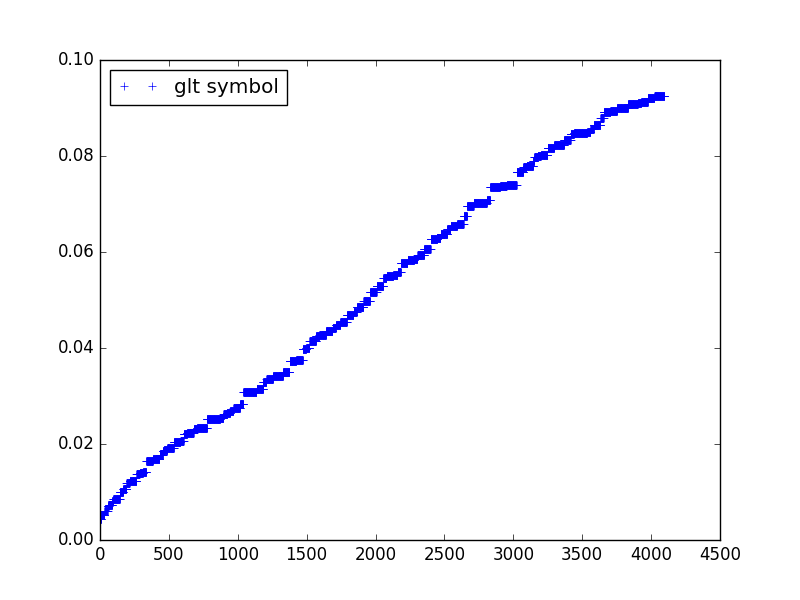
Approximation of the eigenvalues of a (scalar) symbol using an uniform sampling.

User constants and functions

The following example shows how to deal with user defined functions and constants:

>>> def h(x,y):
>>>     return 1 + x**2 + y**2
>>>
>>> discretization = {"n_elements": [16, 16], "degrees": [2, 2]}
>>>
>>> txt  = "alpha * Ni * Nj + h(x,y) * Ni_x * Nj_x + beta * Ni_y * Nj_y"
>>> expr = glt_symbol(txt, dim=2, \
>>>                   verbose=False, evaluate=True, \
>>>                   discretization=discretization, \
>>>                   user_functions={'h': h}, \
>>>                   user_constants={'alpha': 1., 'beta':1.e-3})
>>> print expr
(-32*cos(t1)/3 - 16*cos(2*t1)/3 + 16)*(13*cos(t2)/480 + cos(2*t2)/960 + 11/320)*h(x, y) + 0.001*(13*cos(t1)/480 + cos(2*t1)/960 + 11/320)*(-32*cos(t2)/3 - 16*cos(2*t2)/3 + 16) + 1.0*(13*cos(t1)/480 + cos(2*t1)/960 + 11/320)*(13*cos(t2)/480 + cos(2*t2)/960 + 11/320)

this symbol can be evaluated on a given point:

>>> s = glt_lambdify(expr, dim=2)
>>> s(0.1, 0.1, pi, pi)
0.181580555556

As in the previous example, let’s not evaluate the symbol:

>>> expr = glt_symbol(txt, dim=2, \
>>>                   verbose=False, evaluate=False, \
>>>                   discretization=discretization, \
>>>                   user_functions={'h': h}, \
>>>                   user_constants={'alpha': 1., 'beta':1.e-3})
>>> print expr
alpha*m1*m2 + beta*m1*s2 + m2*s1*h(x, y)

Documentation